Chapter 6: The Normal Distribution

The Normal Distribution

Normal Distribution

Normal Distribution:

• AKA: Gaussian Distribution
• Describes a commonly occurring distribution of the outcomes of random trials

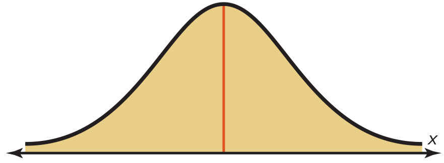
Normal Distribution Curve

Normal Distribution Curve:

• AKA: Bell Curve

• Describes the distribution shape of the normal distribution

  

Standard Normal Distribution

Standard Normal Distribution:

• Universalizes the normal distribution by graphing a normal distributive curve with a mean of 0 and standard deviation of 1.
• Describes continuous distributions
  • As continuous distributions are measured in terms of ranges, rather than individual discrete values, the probability of a range is reflected by the area under the curve between the range limits.
  • Examples:

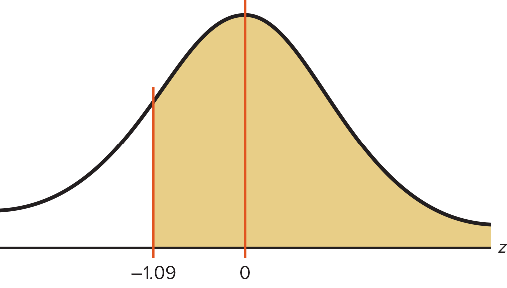
    • To graph of the probabilities of a value being above 1.09 standard deviations below the mean:

      

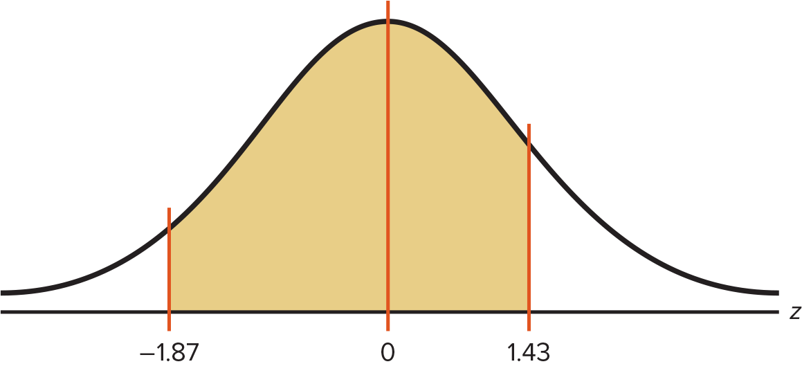
    • To graph the probability of a value being between 1.87 standard deviations below the mean and 1.43 deviations above the mean:

      

Using the Normal Distribution

Z Values

Normal distributions can be scaled to the standard normal distribution by plotting the $z$ value of each outcome.

Z Value:

• Measure of standard deviation units a value is from the mean
• Formula:

To find the value that corresponds to a given Z value:

Empirical Rule

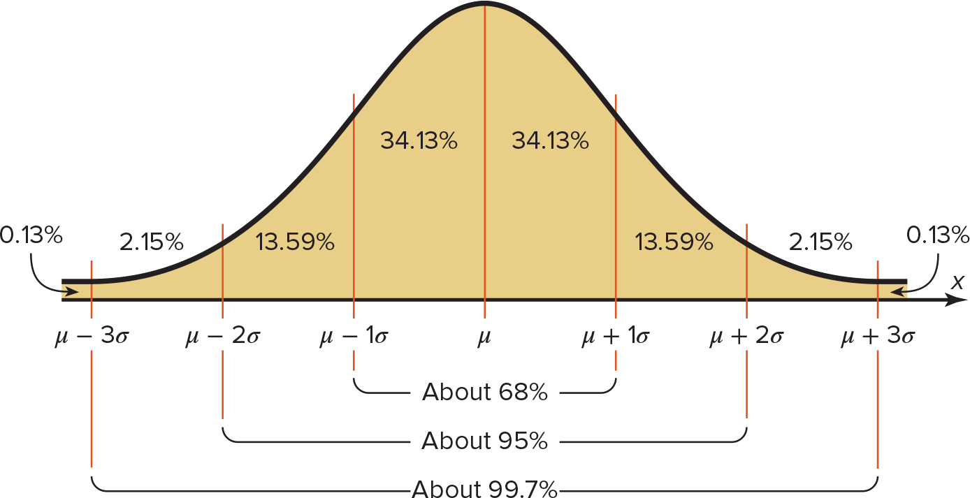
The empirical rule states that in a normal distribution:

• About 68% of outcomes will be within 1 standard deviation of the mean;
• 95% within 2; and

• 99.7% within 3.

  

Standard Normal Distribution Tables

Precalculated tables are used to determine the probability of given standard deviations.

Example A:

• Problem:
  • For a distribution with a mean of 5.2 and a standard deviation of 0.3, find the probability that an outcome will be less than 5.4.
• Solution:
  • First, scale the problem to the standard normal distribution by calculating the $z$ value of 5.4:
    • $\frac {5.4-5.2} {0.3}=0.67$

  • The corresponding graph is:

    

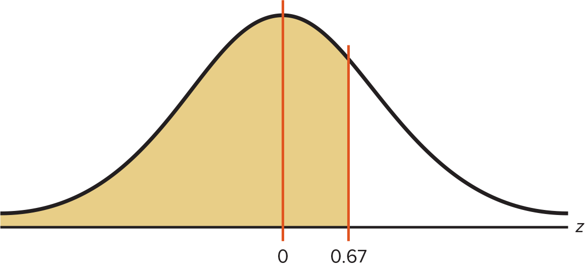
  • Next, use the normal distribution tables to find the area to the left of 0.67.
    • Some tables list the absolute area to the left of a given z value.
      • In such a table, the given value for 0.67 is 0.7486.
    • Other tables list the area between the mean and the deviations from the mean.
      • In such a table, the given value for 0.67 is 0.2468.
      • Since the graph includes the area to the left of the mean, which is 0.5, add 0.5 to the area to the right of the mean, 0.2468, for a result of 0.7486.
• Final Answer:
  • For a distribution with a mean of 5.2 and a standard deviation of 0.3, 74.86% of outcomes will be below 5.4.

Example 2:

• Problem:
  • For a distribution with a mean of 200 and a standard deviation of 20, find the value above which lie 10% of outcomes.
• Solution:

  • First, draw the corresponding graph:

    

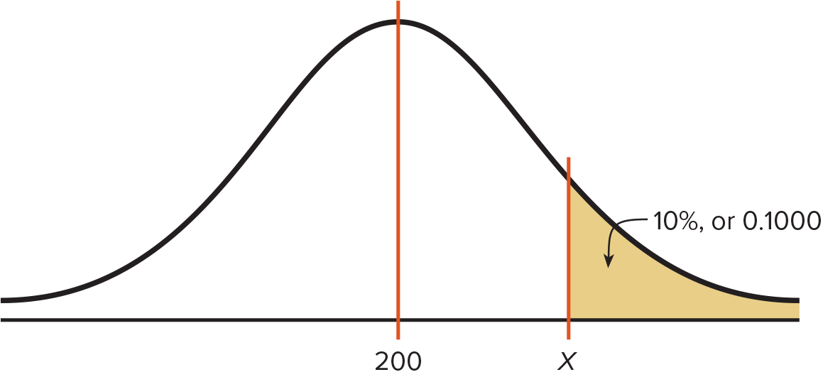
  • Next, find the z value above which lie 10% of outcomes, or, below which lies 90%.
    • The z value with the closest area, 0.8997, is 1.28.
      • (If the requested area is exactly halfway between two z values, use the larger z value.)
  • Finally, scale the z value of 1.28 by multiplying it by the standard deviation.
    • $1.28*20=225.6\approx 226$
• Final Answer:
  • For a distribution with a mean of 200 and a standard deviation of 20, the value above which lie 10% of outcomes is 226.

The Central Limit Theorem

Central Limit Theorem

Central Limit Theorem:

• Describes the distribution of the means of samples of a specific size.

Properties of the Distribution of Sample Means

• If all possible samples of a specific size from a population are measured, the mean of the samples’ means will be the mean of the population.
  • Formula:
  \[\mu _{\bar{X}} = \mu\]
• The mean of individual samples will differ from the mean due to sampling error.
• The standard deviation of the sample means is the standard deviation of the population divided by the square root of the size of the samples.
  • Formula:
  \[\sigma _{\bar{X}} = \frac {\sigma} {\sqrt{n}}\]

• The $z$ value for the probability of the mean of a specific sample be calculated using the above standard deviation formula:

  \[z = \frac{\bar{X} - \mu}{\sigma/\sqrt{n}}\]
• As the sample size increases, the distribution of the samples’ means will more closely resemble a normal distribution.
  • If the population is normally distributed, the sample means will be normally distributed no matter the sample size.
  • If the population is not normally distributed, the sample means are assumed to be normally distributed where $n>30$.

Using the Central Limit Theorem

Where the population is normally distributed or $n>30$, and the population mean and standard deviation are known, the central limit theorem can be used to calculate the probability of the sample mean.

Example:

• Question:
  • For
    • a normally distributed population; with
    • a population mean of 46; and
    • a standard deviation of 3.4,
  • What is the probability that the mean of a sample with 15 elements will be greater than 47.5?
• Solution:
  • To find the solution, we find the $z$ value corresponding to the given sample mean.
  • The formula for a sample mean’s $z$ value takes $\bar{X}, \mu, \sigma$ and $n$.
  • In the example:
    • $\bar{X}=47.5$
    • $\mu = 46$
    • $\sigma = 3.4$
    • $n = 15$
  • Substituting these values in the above formula gives us:
  \[z = \frac {47.5-46} {3.4/\sqrt{15}} \approx 1.7\]
  • Finally, we find the area to the right of $z$=1.7, which is 0.446.
• Answer:
  • There is a 4.46% chance that, in the above scenario, the sample mean will be greater than 47.5.