Chapter 9: Correlation and Regression
Correlation
Correlation
Correlation: The relationship between two variables.
Variable Types:
- Independent Variable:
- Variable that is directly manipulated
- Plotted on the $x$ plane
- Dependent Variable:
- Variable that is not directly manipulated; its value depends on other variables
- Plotted on the $y$ plane
Types of Correlation:
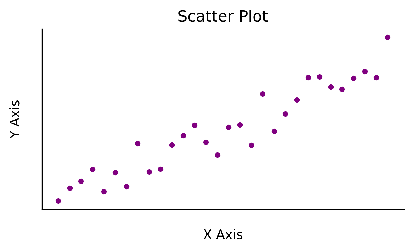
- Positive Linear Relationship:
- When $x$ increases, $y$ increases
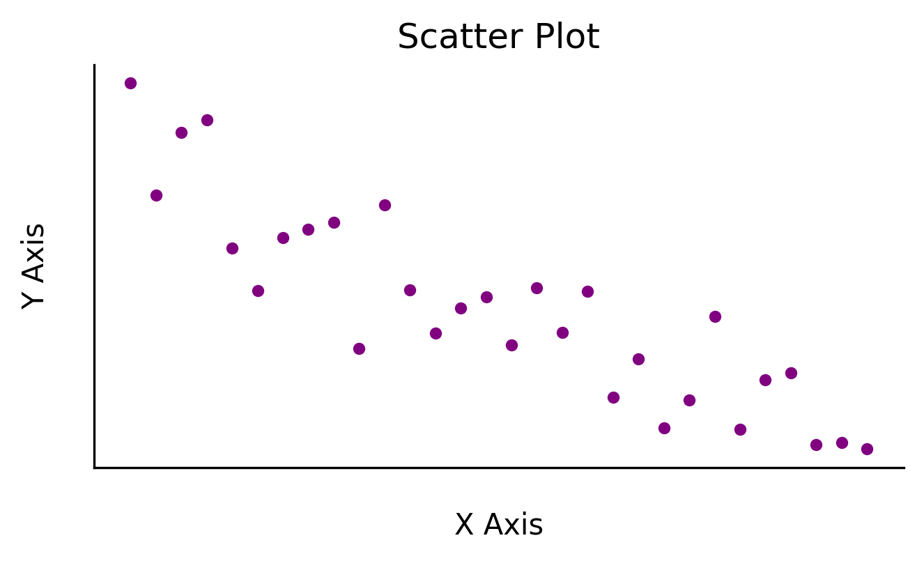
- Negative Linear Relationship:
- When $x$ increases, $y$ decreases
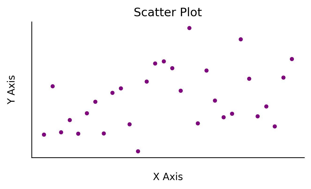
- No Relationship:
- There is no correlation between $x$ and $y$
Correlative Data Descriptive Statistics
Sample correlative data can be organized is a table:
-
Example:
Month Miles Walked; $x$ Pounds Lost; $y$ January 50 4 February 65 4 March 59 4 April 60 3 May 45 6 June 52 2 July 56 6 August 35 7 September 65 4
Scatter Plot
Scatter Plot:
- Graph of ordered pairs of the $x$ independent and $y$ dependent variable values
- Example:
- In the above table, the ordered pairs are {(50, 4), (65, 4)…}.
-
Scatter plot:
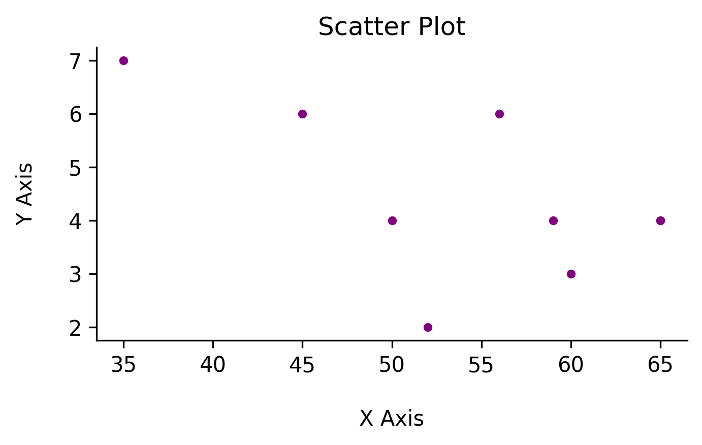
Scatter Plots can visually demonstrate the relationship between variables:
-
Negative Linear Relationship:
-
Positive Linear Relationship:
-
No Relationship:
Correlation Coefficient
Correlation Coefficient
Correlation Coefficient:
- Measure the strength of the relationship between variables
- In statistics, population correlation is generally inferred from sample correlation.
- $\rho$: Population correlation
- $r$: Sample correlation
Pearson product moment correlation coefficient (PPMC):
- Type of correlation coefficient
- Ranges from -1 to 1
- -1: strong negative linear relationship
- 0: no linear relationship
- 1: strong positive linear relationship
Formula for Calculating the Correlation Coefficient
The formula for calculating the correlation coefficient is:
\[r= \frac{n(\Sigma xy)-(\Sigma x)(\Sigma y)}{\sqrt{[n(\Sigma x^2) - (\Sigma x)^2][n(\Sigma y^2)-(\Sigma y)^2]}}\]Setting up a table with the relevant data and sums makes it easier to substitute terms in the equation:
| $x$ | $y$ | $xy$ | $x^2$ | $y^2$ |
|---|---|---|---|---|
| 50 | 4 | 200 | 2500 | 16 |
| 65 | 4 | 260 | 4225 | 16 |
| 59 | 4 | 236 | 3481 | 16 |
| 60 | 3 | 180 | 3600 | 9 |
| 45 | 6 | 270 | 2025 | 36 |
| 52 | 2 | 104 | 2704 | 4 |
| 56 | 6 | 336 | 3136 | 36 |
| 35 | 7 | 245 | 1225 | 49 |
| 65 | 4 | 260 | 4225 | 16 |
| 487 | 40 | 2091 | 27121 | 198 |
Substituting these sums in the above equation gives us:
\[r=\frac{(9\cdot2091)-(487\cdot40)}{\sqrt{[(9\cdot27121)-(487)^2][(9\cdot198)-(40)^2]}}\approx -0.589\]The calculated value for $r$ is -0.589, suggesting a moderate negative correlation.
Testing a Correlation Hypothesis
Correlation Hypothesis
H0 and H1 Hypotheses:
- H0 is the null hypothesis, which is passive and does not make a claim.
- H1 is the alternative hypothesis, which actively makes a claim.
Correlation Coefficient Hypotheses:
- In a correlation coefficient hypothesis, the active claim is that there exists a relationship between the two variables.
- Thus, H0 is that there is no relationship; H1 claims there is:
Testing a Correlation Hypothesis
A correlation hypothesis can be testing using the $t$ value test:
- First, the $t$ value is obtained.
- Next, the corresponding area is retrieved from a $t$ distribution table, and is compared with $\alpha$:
- If the area is beyond $\alpha$, H0 is rejected
- If the area is not beyond $\alpha$, H0 is not rejected
Correlation Coefficient $t$ Value Formula:
-
For a correlation coefficient:
\[d.f. = n-2\] -
The formula for finding the correlation coefficient is:
\[t=r\sqrt{\frac{d.f.}{1-r^2}}\] -
Alternatively, a dedicated PPMC table can be used.
- The PPMC table takes $\alpha$ and $d.f.$ (or $n$) and returns a value that can be directly compared to $r$.
- If $r$ is beyond the value, H0 is rejected, and a linear relationship is accepted.
- If $r$ is not beyond the value, H0 is not rejected.
- The PPMC table takes $\alpha$ and $d.f.$ (or $n$) and returns a value that can be directly compared to $r$.
Example
- Question:
- For the above example data, is $r$ significant for $\alpha=0.05$?
- Answer:
- $r$ was previously calculated to be -0.589.
- For $d.f.=7$ and $\alpha=0.05$, the PPMC table returns a value of: $\pm 0.666$.
- As $r$ is not beyond -0.666, $r$ is not significant, and H0 cannot be rejected.
Regression
Linear Regression
While correlation establishes the strength and direction of the relationship between two variables, regression calculates the actual formula by which one variable can be used to predict the other.
Notation:
- $y’$ is used to represent the predicted value of $y$ based on regression analysis.
Regression Line:
- Line that best fits the scatter plot data
Residual:
- Difference between the predicted $y’$ and the actual $y$.
- The regression line is the line which has the least residuals.
Method of Lease Squares:
- Method of determining the regression line by using the residuals’ squared values
- Example: Would rather a line with 3 points that are all 1 removed than a line with 1 point that is 2 removed
Coefficient of Determination
Coefficient of Determination:
- Percentage of $y$ variability can be attributed to $x$ variability through linear regression.
- Formula: $r^2$
Calculating the Regression Line
The formula for the regression line is given in slope-intercept form:
\[y'=a+bx\]where:
- $y’$ is the predicted $y$ value;
- $a$ is the $y’$ intercept; and
- $b$ is the slope of the line.
The formula for calculating $a$ is:
\[a=\frac{(\Sigma y ) ( \Sigma x ^2) - (\Sigma x)(\Sigma x y )}{n (\Sigma x ^2) - (\Sigma x) ^2}\]The formula for calculating $b$ is:
\[b = \frac {n(\Sigma x y ) - ( \Sigma x ) ( \Sigma y )}{n (\Sigma x ^2) - (\Sigma x) ^2}\]Example
- Question:
- For the above data, calculate $y$ for $x=51$.
- Answer:
-
Substituting the above values in the formula for $a$ gives us:
\[a= \frac { (40*27121)-(487*2091)}{(9*27121)-(487)^2} \approx 9.613\] -
Substituting the above values in the formula for $b$ gives us:
\[b = \frac { (9*2091)-(487*40)} {(9*27121)-(487)^2} \approx -0.096\] -
Resulting in a linear regression line of:
\[y'=9.613-0.096x\] -
Calculating for $x=51$ result in:
\[y' = 9.613-(0.096*51)=4.717\]
-
Critical Value for PPMC Chart
| d.f. ( n-2) | 0.1 | 0.05 | 0.02 | 0.01 |
|---|---|---|---|---|
| 1 | 0.988 | 0.997 | 0.9995 | 0.9999 |
| 2 | 0.9 | 0.95 | 0.98 | 0.99 |
| 3 | 0.805 | 0.878 | 0.934 | 0.959 |
| 4 | 0.729 | 0.811 | 0.882 | 0.917 |
| 5 | 0.669 | 0.754 | 0.833 | 0.874 |
| 6 | 0.622 | 0.707 | 0.789 | 0.834 |
| 7 | 0.582 | 0.666 | 0.75 | 0.798 |
| 8 | 0.549 | 0.632 | 0.716 | 0.765 |
| 9 | 0.521 | 0.602 | 0.685 | 0.735 |
| 10 | 0.497 | 0.576 | 0.658 | 0.708 |
| 11 | 0.476 | 0.553 | 0.634 | 0.684 |
| 12 | 0.458 | 0.532 | 0.612 | 0.661 |
| 13 | 0.441 | 0.514 | 0.592 | 0.641 |
| 14 | 0.426 | 0.497 | 0.574 | 0.628 |
| 15 | 0.412 | 0.482 | 0.558 | 0.606 |
| 16 | 0.4 | 0.468 | 0.542 | 0.59 |
| 17 | 0.389 | 0.456 | 0.528 | 0.575 |
| 18 | 0.378 | 0.444 | 0.516 | 0.561 |
| 19 | 0.369 | 0.433 | 0.503 | 0.549 |
| 20 | 0.36 | 0.423 | 0.492 | 0.537 |
| 21 | 0.352 | 0.413 | 0.482 | 0.526 |
| 22 | 0.344 | 0.404 | 0.472 | 0.515 |
| 23 | 0.337 | 0.396 | 0.462 | 0.505 |
| 24 | 0.33 | 0.388 | 0.453 | 0.495 |
| 25 | 0.323 | 0.381 | 0.445 | 0.487 |
| 26 | 0.317 | 0.374 | 0.437 | 0.479 |
| 27 | 0.311 | 0.367 | 0.43 | 0.471 |
| 28 | 0.306 | 0.361 | 0.423 | 0.463 |
| 29 | 0.301 | 0.355 | 0.416 | 0.456 |
| 30 | 0.296 | 0.349 | 0.409 | 0.449 |
| 35 | 0.275 | 0.325 | 0.381 | 0.418 |
| 40 | 0.257 | 0.304 | 0.358 | 0.393 |
| 45 | 0.243 | 0.288 | 0.338 | 0.372 |
| 50 | 0.231 | 0.273 | 0.322 | 0.354 |
| 60 | 0.211 | 0.25 | 0.295 | 0.325 |
| 70 | 0.195 | 0.232 | 0.274 | 0.302 |
| 80 | 0.183 | 0.217 | 0.256 | 0.284 |
| 90 | 0.173 | 0.205 | 0.242 | 0.267 |
| 100 | 0.164 | 0.195 | 0.23 | 0.254 |